
Control engineering, one of the most relevant developments of the 20th century, has many particularities that result somehow strange from the perspective of a computer science student, especially when he/she confronts it for the first time. For instance, it is difficult to assimilate the fact that in a system block diagram all the signals exist at the same time (a computer scientist is told to consider sequential operations when using diagrams similar to that; it is common to consider that each signal is updated only after the subsystem that produces it finishes its internal work).
These problems get worse when, for the sake of devoting enough space in textbooks to explain the numerous complexities of the discipline, some of the most basic concepts are often just mentioned, without demonstration or even discussion. (Ok, well, that is a general problem with scientific writing that bothers me in a particular manner U_U )
Two entangled and shallowly explained concepts in control engineering are whether the derivative of a signal is a causal operation and whether it is realizable. Common answers in the Internet often miss the point, even experienced people find difficult to give a clear and direct answer for this, most textbooks just mention the fact without elaborating it… A hell of an educational nightmare, from my modest point of view.
Here I will try to give an answer from a rather innocent, newcomer (but mathematically educated) perspective. Let’s see if I am able to provide a straight enough explanation… or just contribute with more darkness to the nightmare 😉
1. First of all: when is a system causal?
(Considering a system as something that processes signals to produce new signals; furthermore, considering only SISO continuous-time systems, i.e., those that take a Single continuous-time signal as Input and yield a Single continuous-time signal as Output).
Well, we can define a system as causal iff the signal that it produces is formed just through the use of present and past values from the signal that it receives. Such a system cannot read the future, as it seems logical for physical processes.
From that definition: is it causal a system that derives its input signal? (is the derivative of a function a causal operation?)
Let’s see. The derivative of a function f(t) is formally defined as another function:
\frac{df(t)}{dt} = lim_{h \to 0} { \frac{f(t+h) - f(t)}{h} }
If the derivative exists (is well defined and has some finite value), the limit above exists, which implies that both its left and right limits exist and their values coincide:
\frac{df(t)}{dt} = lim_{h \to 0^{+}} { \frac{f(t+h) - f(t)}{h} } =
= lim_{h \to 0^{-}} { \frac{f(t+h) - f(t)}{h} }
Since we are dealing with real, physical systems and signals, that cannot change their behaviour abruptly in zero time (i.e., that need to change through a sequence of infinitesimal changes), we will assume that, indeed, both limits above exist and coincide, i.e., that the derivative of a continuous-time signal produced by a physical system exists at any time. Mathematically, as it has been kindly pointed out to me by Dr. Luigi Lannelli, we will consider here signals that belong to C^{1}, or, for the sake that they can be differentiated sequentially more than once, to C^{\infty}.
But if the derivative exists, it could be calculated, for instance, with the second limit we have noted previously. Since that limit only uses values of time at present (t) or before (t+h, h \text{ negative}), it must be that, by using the second limit, differentiation is causal. Since the value of the second limit must coincide with the one yielded by the first limit, we must conclude that differentiation is causal for physical signals.
In some places one can read that the derivative is not causal (i.e., it is considered to be uncausal) because it “looks at” the future of the signal, and looking at the future cannot be a causal operation. Oook, I have to admit that I have used that reasoning sometimes (years ago! the offense has prescribed!). But what the derivative does is to estimate or predict the value of the signal at a future time. It does not know that future nor accesses it in any way. More concretely, if we know the derivative at time t, we know how the signal is changing at that time (i.e., at present), and, with that, we can approximate the value of the signal at some specific future time t+h, h \text{ positive}, for example linearly. It is true that the approximation will be better as h gets smaller, but it will never be guaranteed to be the actual value, since this procedure is not looking at the future in any way (it just gives us a hint). We cannot use that reason to establish the causality of differentiation.
2. Now for the second big question: is the derivative realizable?
As before, we need to provide some definition for realizability. In the context of physical systems, realizability is the property of having some way of implementing a mathematically specified system with physical components. So, can differentiation be implemented with physical components? Notice that, due to their physical nature, realizable systems must be causal. What we wonder here is whether the reverse is also true.
The answer for differentiation is no, and although in some places you will read that this happens because the derivative has an unbounded gain at high frequencies{}^{note} (which is true, but also overwhelming if it is read in the first pages of a textbook by a newcomer to Control Engineering), it is due, basically, to the following, much more understandable reason: a physical system cannot provide infinite energy. [{}^{note:} Mathematically, its transfer function tends to \infty as s \rightarrow \infty, i.e., it has poles at infinity, which, in addition, makes it BIBO unstable].
Since any input signal, even being bounded in magnitude, can have an arbitrarily large derivative (when the magnitude changes too rapidly), implementing an exact differentiation would force the system to use arbitrarily large amounts of energy. Therefore, it cannot be realizable, at least, in an exact form and for all situations.
Furthermore, the input signal has noise, that is unavoidable in practice. Noise consists of (very informally) unpredictable oscillations superimpossed to the main trend of the signal, with low magnitude but high frequency. The problem here is high frequency and unpredictable: the larger the changes in magnitude due to noise, in a given, short time, the larger the derivative. No matter how small is the magnitude of the noise: if that noise changes rapidly (i.e., its frequency is high), it will have large derivatives. And, unfortunately, we cannot take them into account before operation for all circumstances, because noise, by definition, is unpredictable. Moreover, we cannot get rid of noise (e.g., through filtering) without incurring in other problems, mainly the induction of delays.
At this point, some readers (hello you two!) may complaint: “Hey, wait a minute! I know of some physical system that implements differentiation“. Certainly you know. For example:
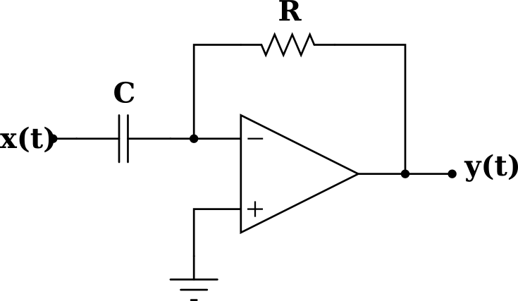
In theory, this Operational Amplifier circuit is a system that implements the following transformation of the input voltage:
y(t)=-RC\frac{dx(t)}{dt}
But, again, in the real world things are more complicated than when sketched on paper: that OpAmp needs an external power source to work (typically, \pm15v) that is bounded in the amount of energy it can provide to the circuit, in particular to the output signal y(t). Therefore, if the input signal has high frequency noise or its main trend changes too quickly, the output will be clamped and no longer equal to the derivative. Maybe you consider this to happen only sporadically, but its effects in a real controller can be catastrophic.
Consider this other example, one of the most simple you can figure out, also electrical:
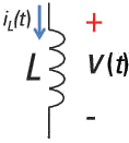 In theory, it must be that:
However, again, that is only a theoretical inductor. A physical inductor is limited in the magnitude of the difference of voltage that it can cope with (or, if you prefer, in the magnitude of the current changes).
I am almost finished. However, since I am a computer scientist and this post is intended (mostly) for computer science students, I cannot leave it here without some words about computational implementations. Even if we try to implement differentiation in a computer, e.g., in an embedded controller, the situation gets no much better: in a CPU the derivative must be approximated by discrete numbers (yes, even when you program in C and are so lucky to have support for floats), which means that we have bounds, like in the physical world, on the large those numbers can be, but also on their resolution. For example, we can use the Euler method with some small positive h to implement an approximation to the derivative:
\frac{dx(t)}{dt} \approx \frac{x(t)-x(t-h)}{h}
but notice that, if h is too small in order to have a good approximation, the numerical result can easily overflow the computer number capacities. Still worse: we will get more of the high frequency characteristics of the input signal as we set higher the frequency of sampling (smaller h), making the derivative, therefore, potentially larger. Much worse! the program must now run fast enough to do all its periodical calculations, including that approximation of the derivative, in less than h units of time, if we want to provide the hard real-time performance needed for controlling a critical system…
So yes, we can implement the Euler method in a computer, and make it work ok under suitable trade-offs, but certainly it is not a general, complete, exact realization of differentiation.
3. (ADDENDA) What about the integral?
Well, it is straightforward to see that a system that integrates its input is causal: in order to integrate, it just uses the past and present of the input signal.
However, in its implementation we found similar problems to those commented above about the derivative. The integral is an accumulation of the area delimited by the input signal. Depending on the signal, that area can become arbitrarily large even when the signal is bounded in magnitude: just think of a constant input, whose integral will tend to infinite over time. Since no physical system is able to provide infinite energy, integration is not realizable physically in the general case.
Note, however, that in the case a system always work with bounded signals, it is guaranteed that any integration it performs will not be unbounded. That is the reason why integrators are preferred to differentiators when realizing physical systems.
As before, you certainly know some physical “integrators”. Maybe the most simple in the electrical domain is this:
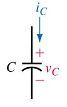 Theoretically, it satisfies the following equation:
Alas, that is only theory! A real capacitor is limited in the magnitude of the difference of voltage it can cope with, thus we reach the same limitation as with “physical differentiators”. (There are also “integrator” circuits based on OpAmps; of course, subjected to the same kind of physical limits).
In the case of a computer implementation of the integral, the situation only changes with respect to that of differentiation in that integration does not amplify noise (large derivatives of the inputs are not translated into the output), although, in return, it amplifies the errors due to the numeric system of a computer (based ultimately on integers) step by step, through their progressive and potentially dangerous accumulation, producing in the long term an output signal that may be far from the real integral (this gets worse when we set up more than one integrator in series).
In short: only in particular situations where we are absolutely sure that the integral of the input signal will be bounded over time and, in the case of a computer implementation, that the accumulation of errors will not be an issue, we can say that we can realize integration.